Adam (L2 regularization) 和 AdamW（weight decay）

读这篇博客的基础：

​ 需要懂梯度下降的优化算法，特别是SGD,以及SGD+momentum.

读完本篇博客可以了解到：

​ Adam的实现过程

​ AdamW和原来Adam+ L2 regularization的区别

​ AdamW的实现过程

1. Adam 详细过程

Adam全称是Adaptive Moment Estimation。是一种自适应调节学习率的优化算法。

Whereas momentum can be seen as a ball running down a slope, Adam behaves like a heavy ball with friction, which thus prefers flat minima in the error surface

我们来看看Adam的具体过程。

SGD

首先我们来看一下SGD的过程,在梯度下降的过程中，对目标函数/（深度学习中为损失函数），更新参数： \(\theta = \theta - \eta \cdot \nabla_\theta J( \theta)\) $J(\theta)$是objective function.如果是SGD,那么输入就是单个训练数据$[x(i);y(i)]$，来更新参数： \(θ=θ−η⋅∇θJ(θ;x(i);y(i))\)

Adam

再来看Adam和普通的SGD有什么区别。对目标函数$J(\theta)$求导，可以得到导数$g_t(\theta)$,接下来我们就根据导数来计算。 \(m_t &= \beta_1 m_{t-1} + (1 - \beta_1) g_t \\ v_t &= \beta_2 v_{t-1} + (1 - \beta_2) g_t^2\)

• $m_t$是estimates of the first moment (the mean) of the gradients. 初始值$m_0=0$

• $v_t$是estimates of the second moment (the uncentered variance) of the gradients. $v_0=0$

为了避免翻译的歧义，我直接放原文。这些表示啥都不重要，你只需要知道一项是和导数$g_t$有关，一项是和导数$g_t^2$有关。初始值都为0。因为是导数的估计，所以也是Adam名字的由来。

下一步是debiasing step, 因为上述两个estimation $m_t, v_t$的初始值都是0，所以在刚开始的时候他们都偏向（bias）于0附近。所以需要去偏置。（As $m_t$ and $v_t$ are initialized as vectors of 0’s, the authors of Adam observe that they are biased towards zero, especially during the initial time steps, and especially when the decay rates are small (i.e. $β_1$ and $β_2$ are close to 1).） \(\hat{m}_t &= \dfrac{m_t}{1 - \beta^t_1} \\ \hat{v}_t &= \dfrac{v_t}{1 - \beta^t_2} \\) 接下来就是更新参数$\theta$，通过类似于RMSprop里面的操作，结合$\hat m_t$和$\hat v_t$: \(\theta_{t+1} = \theta_{t} - \dfrac{\eta}{\sqrt{\hat{v}_t} + \epsilon} \hat{m}_t\) $\epsilon$一般设置为1e-8, $\eta$是学习率。上面就是Adam的全部过程。

2. Adam + L2 regularization

一般来讲，在深度学习的优化过程中，L2正则化是直接给目标函数或者说损失函数的。

在分类的例子中（一般比较离散化）,假设用MSE作为评价标准,L2正则化表示为： \(Loss = J(\theta) = MSE(\hat y, y) + wd * sum(\theta ^2)\) wd是weight decay的系数。$\theta$要平方是因为是L2 norm。

在拟合的例子中（一般是连续的问题）： \(Loss = J(\theta) + wd * sum(\theta ^2)\)

在一般的SGD下，通过对Loss求导，离散数据下是差分。在梯度下降的过程中，第t次更新参数： \(\theta (t) = \theta (t-1) - \eta * \frac {dLoss}{d \theta}\)

所以 \(\theta (t) = \theta (t-1) - \eta* \nabla_\theta J( \theta) - \eta *2wd*\theta\) 上述的公式，刚刚好就是weight decay的方法: 在更新参数的时候，对参数权重weight, 直接作用。在每次更新参数的时候，都会比一般Gradient Descent的方法多了一个 $2wd*\theta$的项，因为是一开始（original weight）到最后weight收敛，都会减去这个常数项。所以是weight decay.

从上面的过程可以看出L2 regularization 和weight decay两者在一般的SGD中，是等价的。

3. Adam + L2 和 Adam + weight decay(AdamW)的不同

但是对于比较复杂的梯度下降方法，L2 regularization的方法，是不能推导得到和weight decay等价的。比如momentum这个相对Adam更加简单的方法，也是不能用，从侧面也可以说明Adam这种更复杂的方法不能使得L2和weight decay不等价，momentum的过程： \(\begin{align} \begin{split} v_t &= \gamma v_{t-1} + (1- \gamma) \nabla_\theta J( \theta) \\ \theta _{t} &= \theta _{t-1} - \eta*v_t \end{split} \end{align}\) 这个$v_{t-1}$就是上一步的梯度值。相当于保持原来下降的方向。

weight decay: \(\theta _{t} = (1-\eta(1-\gamma) *2wd)*\theta _{t-1} - \gamma \eta v_{t-1} - \eta(1-\gamma) \nabla_\theta J( \theta)\) L2 regularization: \(Loss = J(\theta) + wd * sum(\theta ^2) (在loss处直接做weight decay)\) 根据momentum更新参数的公式： \(v_t &= \gamma v_{t-1} + (1-\gamma) \nabla_\theta [J(\theta) + wd * sum(\theta ^2)] \\ \theta &= \theta - \eta v_t\)

从上述两个公式来看，momentum优化算法下的L2 regularization 和 weight decay是不一致的。

至于Adam的推导就更不必说了。

Adam实现过程：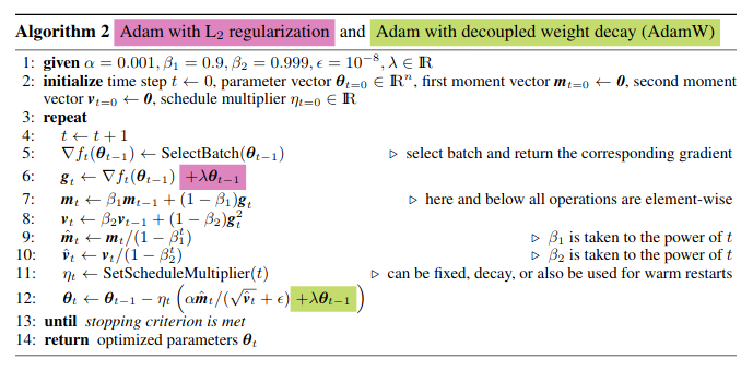

再放两张torch实现的对比

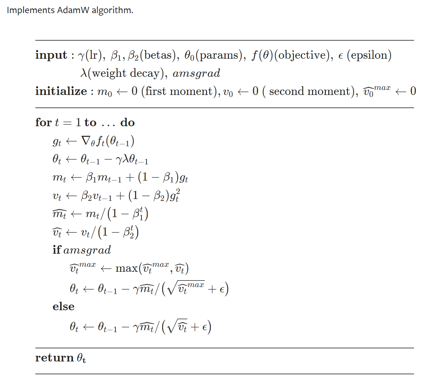
图中的 amsgrad是在计算Adam时，得到$ \hat{v}t$那一步，比较$ \hat{v}_t$何$ \hat{v}{t-1}$的大小，保留大的那个。这是为了防止Adam到后面lr越来越小。停留在局部最优点。

参考

https://www.fast.ai/2018/07/02/adam-weight-decay/

https://ruder.io/optimizing-gradient-descent/index.html#fn20

https://pytorch.org/docs/stable/optim.html